Introduction: A snack food making company has gathered data from its customers about whether they like the product or not they make and if they like which version they prefer between version 1 and version 2, and also about the money they would like to spend on that product. The investigation on the customers’ preference and their willingness to spend on the product is based on a large hypothetical data set. Among this large population each of us (student) has to work with the separate sample, each consisting of 100 individual. The company gathers the data for following two hypothesis to be tested:
- Is the proportion of people that prefer version 2 significantly different to 50%?
- Is the mean of the variable “How much they would pay” significantly different to $2?
The problems of getting survey data in the real world: The data used in the assignment is not real world data. We have used hypothetical data to investigate our research questions. Because there are many problems of getting survey data in the real world. Survey data collection methods are time consuming and costly. Also lack of proper training period for the data collectors could create several problems like misunderstanding, misconception and biasness during the data collection process. That’s why sometimes we create hypothetical data through simulation instead of collecting real world data.
But if we have to collect the survey data we would be needing proper data collection methods, instruction form an experience person in that field and proper training period and guidance for the filed workers who would collect data from the respondents.
Description of Data set: There are 1000 samples of size 100 on the peoples’ preference on the product made by the company. Among them 60040 persons liked the product and 39960 persons didn’t.
We, each of the students are given a separate sample to analyze with. Each sample data set contains 100 observations on 6 variables- Gender, do they like the product, which version is the best, how much they would pay, are they old, income. Among these variables “how much they would pay” and “income” are the numerical variables and rest of them are categorical variables.
Summary of the data set: Numerical and graphical summary of the variables are given below through univariate and bivariate descriptive statistics, histograms and bar diagrams.
- i) “Income”:
Descriptive statistics:
| Minimum: | 45000 |
| Maximum: | 80000 |
| Range: | 35000 |
| Count: | 100 |
| Sum: | 6217000 |
| Mean: | 62170 |
| Median: | 63000 |
| Mode: | 63000 |
| Standard Deviation: | 10200 |
| Variance: | 104100000 |
| Quartiles: | Quartiles: Q1 –> 53000 Q2 –> 63000 Q3 –> 70000 |
| Skewness: | 0.05892 |
| Kurtosis: | 1.823 |
Descriptive statistics shows that average income of the 100 sample respondents is $62170 with standard deviation is equal to 10200. And among that $45000 is the lowest income and $80000 being the highest income.
Histogram: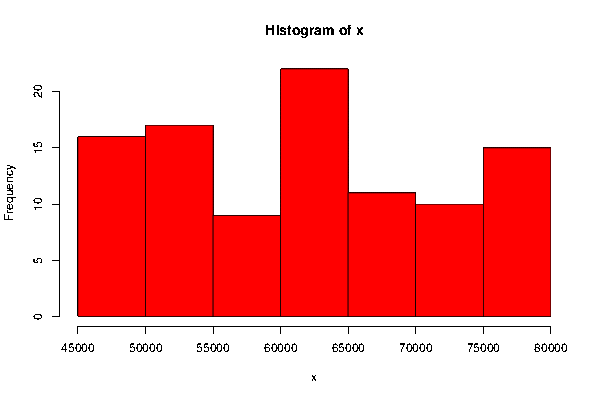
The histogram of the variable “Income” shows that the highest frequency occurs with the class $60000-$65000 that is, highest number of respondents have income in that class. And the distribution of the variable “Income” isn’t normally distributed.
- ii) “How much they would pay”:
Descriptive statistics:
| Minimum: | 0 |
| Maximum: | 3.3 |
| Range: | 3.3 |
| Count: | 100 |
| Sum: | 249.1 |
| Mean: | 2.491 |
| Median: | 3.1 |
| Mode: | 3.3 |
| Standard Deviation: | 1.249 |
| Variance: | 1.561 |
| Quartiles: | Quartiles: Q1 –> 0.5 Q2 –> 3.1 Q3 –> 3.2 |
| Skewness: | -1.273 |
| Kurtosis: | 2.676 |
Descriptive statistics shows that average amount of money people would like to spend on the product is $2.491 with standard deviation is equal to 1.249. And among the respondent someone would prefer to spend no money on the product (minimum is $0) and some people would like to spend maximum $3.3.
Histogram: 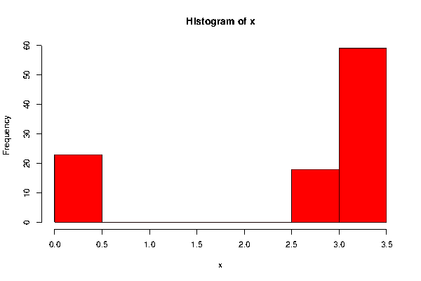
The histogram of the variable “How much they would pay” shows that the highest frequency occurs with the class $3-$3.5 that is, highest number of respondents want to spend $3-3.5 on the product. Also it is noticeable that no respondent wants to spend between $0.5-2.5. And the distribution of the variable “Income” isn’t normally distributed.
- Descriptive bivariate and graphical summary:
- “Gender” and “Do they like the product”:
| sample collector id |
|
|||
| Count of do they like the product? | Column Labels | |||
| Row Labels | Like | Hate | Grand Total | |
| female | 26 | 14 | 40 | |
| male | 35 | 25 | 60 | |
| Grand Total | 61 | 39 | 100 |
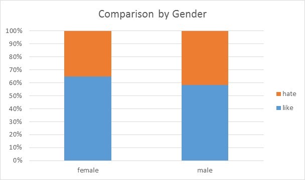
The bar diagram shows that 65% of the females like the product and 58% of the males like the product. That means, female respondents preferred the product than male respondents.
- “How much they would pay” and “Gender”:
Numerical summaries of the females among people who would pay:
| Minimum: | 0 |
| Maximum: | 3.3 |
| Range: | 3.3 |
| Count: | 40 |
| Sum: | 112.2 |
| Mean: | 2.805 |
| Median: | 3.1 |
| Mode: | 3.3 |
| Standard Deviation: | 0.9679 |
| Variance: | 0.9369 |
| Quartiles: | Quartiles: Q1 –> 3 Q2 –> 3.1 Q3 –> 3.2 |
| Skewness: | 0.2 |
| Kurtosis: | 2.963 |
The numerical summaries shows that female are willing to spend on average $2.805 on that product.
Numerical summaries of the males among people who would pay:
| Minimum: | 0 |
| Maximum: | 3.3 |
| Range: | 3.3 |
| Count: | 60 |
| Sum: | 136.9 |
| Mean: | 2.282 |
| Median: | 3.1 |
| Mode: | 3.3 |
| Standard Deviation: | 1.374 |
| Variance: | 1.888 |
| Quartiles: | Quartiles: Q1 –> 0.4 Q2 –> 3.1 Q3 –> 3.2 |
| Skewness: | 00.8663 |
| Kurtosis: | 1.781 |
The numerical summaries shows male are willing to spend on average $2.282 on that product. That mea
Back to back histogram to compare the amount male and female would pay for that product: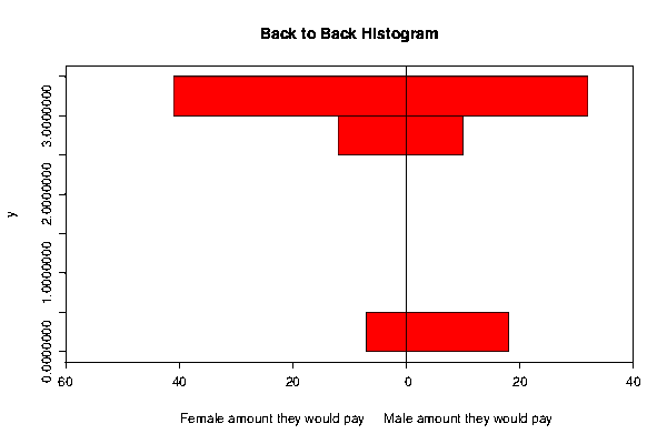
Back to back histogram indicates that female prefer to spend more money on the product than by the male.
Confidence interval for proportion and mean:
- 95% confidence interval for the proportion of people that prefer version 2 is given by:
P {p^ -Z S.E (p^)} = 1-0.05
Here, n=61; Zα/2 =1.96; p^ = ; S.E (p^) =
= 0.62 = = 0.0621
So,
P {0.62-1.96*0.0621 p }= 0.95
=> P {0.50 p } = 0.95
So, {0.50, 0.74} is the 95% confidence interval for the population proportion of people that prefer version 2.
- 95% confidence interval for the mean of the variable “How much they would pay” is given by:
P { – Z*S.E ()} =1-0.05
Here, n=61; Zα/2 =1.96; 2.498360656; = = = 0.16004596
So,
P {2.498360656 – 1.96*0.16004596 } = 0.95
=> P {2.1847 } = 0.95
So, {2.1867, 2.8121} is the 95% confidence interval for the mean of the variable “How much they would pay”.
Hypothesis Testing:
- The null hypothesis is, P= 0.50
against,
alternative hypothesis, P≠ 0.50
The test statistic is given by,
Z= ~ N (0, 1)
Here, n=61; P= = = 0.6229
So, Z= = 1.9197
This is the calculated value of Z.
And the tabulated value of Z at 5% level of significance is obtained from the standardized normal distribution table as 1.96.
Since the calculated value doesn’t exceed the tabulated value we may conclude that the null hypothesis is accepted at 5% level of significance. Hence, the claim, proportion that prefer version 2 is different to 50% is not significant enough, i.e. isn’t true at 5% level of significance.
- The null hypothesis is, µ = $2
against,
alternative hypothesis, µ ≠ $2
The test statistic is given by,
Z= ~ N (0, 1)
= = 3.1138
This is the calculated value of Z.
And the tabulated value of Z at 5% level of significance is obtained from the standardized normal distribution table as 1.96.
Since the calculated value exceeds the tabulated value we may conclude that the null hypothesis is rejected at 5% level of significance. That is, we may claim that the mean of the variable “How much they would pay” is different to $2 at 5% level of significance.
Disadvantages of Quantitative methods: Quantitative methods are rigid and provides less detail on the motivational, attitudes and behavioral study subjects. The findings of quantitative research methods are numerical and therefore lack a detailed narrative of human perception. The respondents may also provide answers that reflect their preconceived hypothesis.
In social and behavioral science research study qualitative research is more appropriate than the quantitative research, since qualitative research deals with the people’s opinion and behavioral type questions.
Conclusion: The concept of the assignment was to use a hypothetical data set to make inferences/decisions about a real world business scenario. In the previous sections of the assignment we have got familiar with the problem of getting survey data in the real world. We also have got familiar with the sampling distribution of an estimate. We have drawn inferences about a large population (100000) from a small sample of size 100. Numerical and graphical summary of the data was done using univariate and bivariate descriptive statistics as well as bar diagram, histogram and back to back histogram.
Inferences about the population parameters were also drawn using the confidence intervals. The research questions of the assignment was that a snack food making company wanted to know if the proportion of people that prefer version 2 of the product is significantly different to 50% and also if the mean of the variable “How much they would pay” is significantly different to $2. And simple hypothesis testing concludes that the first claim isn’t significantly true and the second claim is significantly true, i.e. version 2 isn’t significantly preferred over version 1 and people would pay significantly different than $2. We have also discussed the disadvantages of quantitative research in social and behavioral science and the use of qualitative research in that area.
